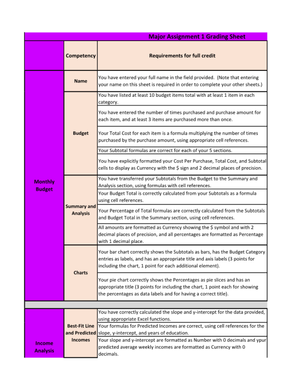
Assignment Advisory: You must use the latest desktop version of Excel for Microsoft 365 for this assignment. (This is provided free by GCU; contact the Help Desk for more information and help installing the software.) Using an earlier version of Excel or a different spreadsheet program may result in missing or corrupted template elements.  Copying cells from or into this template may likewise result in corrupted data.

1. Enter your full name in the blue-shaded area here.  If your full name is less than 5 letters long, add additional letters 'X' at the end until you reach length 5
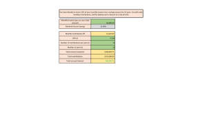
2. Below, you will develop a simplified monthly budget, including entries for 5 separate categories as given.  You must enter at least 10 budget items total across all categories, with up to 5 entries per category.  Each category must include at least one budget item.  For at least 3 budget items, the number of times purchased per month must be greater than 1.  Format all costs as Currency with 2 decimal places.
3. Here, use Excel formulas to transfer the subtotals and total from your budget into this table, and then calculate the percentage of the budget total represented by each category.  Format the costs as Currency with two decimal places of precision and the percentages as Percentage with one decimal place of precision.
4. Below you will insert two charts for this data.  First, insert a bar chart that shows each Subtotal amount as a bar, has the Budget Categories as bar labels, changes the chart title from the default, and adds axis titles for both axes.  Then, insert a pie chart that shows the percentage of the Budget Total represented by each Budget Category based on the Percentage of Total column, changes the chart title from the default, and includes the percentages as data labels.
5. On this sheet, you will investigate the relationship between years of education and average income.

• First, consider the following chart of education versus average income.  Below it, use the built-in Excel functions SLOPE() and INTERCEPT() to find the slope and y-intercept of the best-fit line for the given data.  Then, to the right, use the slope and y-intercept to calculate the average weekly income for all years of education from 8 through 24.  Finally, create a chart showing the BLS data as a scatterplot, and add a trendline to this chart showing years of education versus predicted average income superimposed on the BLS data and forecasting backward to 8 years and forward to 24 years.  (That is, the line should start at 8 years and end at 24 years on the horizontal axis.)
• Here, you should format your slope and y-intercept as numbers with 0 decimal places and your average weekly incomes as Currency with the $ symbol and 0 decimal places.
• In case you'd like to explore the data, numbers here are derived from Bureau of Labor Statistics figures at https://www.bls.gov/emp/tables/unemployment-earnings-education.htm.  However, you don't need to take any steps related to this reference for the assignment."

6. Add your chart here: an XY-scatterplot of the BLS Data in columns A and B (NOT the data in columns C and D) plus an auto trendline forecasting backward to 8 and forward to 24 years
7. On this sheet, you will consider several conversions related to calculations you might see in a professional context.  For each conversion, you'll identify and apply appropriate ratios to yield the given result.  Remember that ratios can use either unit over the other, and that you should order ratios so that units cancel in the numerator and denominator for intermediate steps.

First, examine this conversion factor table; you will use conversion factors from this table in your formulas in part 8.  Note that if you use a ratio of the Second Units over the First Units, then your multiplier will be the conversion factor itself; on the other hand, if you use a ratio of the First Units over the Second units, then your multiplier will be 1 divided by the conversion factor.  For example, when multiplying by lb/kg, you would multiply by F4 or F4/D4; when multiplying by kg/lb, you would multiply by 1/F4 or D4/F4."

8. Now, use entries from the conversion table to perform the following conversions.  Note that you may use entries only from the table above, even if a more direct conversion is possible.  For each part, the number of ratios required is shown in the table.  Note that your ratios for the formulas may be either one of the conversion factors above (like =F10 or =F10/B10) or the reciprocal (like =1/F9 or =B9/F9), as illustrated in the example.  No special formatting is required for the cells containing your formulas.  In the blue cells, enter the ratio of units that you multiplied by for each conversion. You should use the abbreviations provided above, including capitalization as given.
9. Some conversions use ratios plus another additive term (summand).  Here, you'll convert from Fahrenheit to Celsius and from Celsius to Fahrenheit, using the following symbolic formulas:

1. Celsius to Fahrenheit:   F = (9/5)*C + 32
2. Fahrenheit to Celsius:   C = (5/9)*(F - 32)

Use formulas to populate the two empty cells below: specifically, you should convert the value in from Fahrenheit in B26 to Celsius in E26 and from Celsius in E27 to Fahrenheit in B27.  No special formatting is required for your cells here.  Note that you may NOT use a built-in Excel function for your conversions."